Here we will explore how to use the Theano and Keras Python frameworks for designing neural networks in order to accomplish specific classification tasks.In the process, we will see how Keras offers a great amount of leverage and flexibility in designing neural nets.In particular, we will examine two active areas of research: classification of textual and image data.
The Theano Framework
Theano was originally developed as a symbolic math processor at the University of Montreal, for the purpose of performing symbolic differentiation or integration, on complicated non-linear functions.The University of Montreal offers many learning resources for Theano and its spin-off frameworks of Keras, Blocks, and Fuel.The reader is encouraged to explore their resources and summer school 2015 course content.
The symbolic math processing feature of Theano gives it a similarity to Mathematica, or Maple.However, the Theano interface is lower-level, since Python is a scripted programming language.In Theano, functions are represented symbolically, but they can also be evaluated at coordinates, producing numerical values.Theano can be used for solving problems outside the realm of neural networks, such as logistic regression.Because Theano computes the gradient symbolically, it removes the chance of errors arising from determining an analytic form of the gradient by hand, and then translating it into code.Since Theano makes use of GPUs for computation in general, other types of machine learning approaches, outside of the scope neural networks, can also realize performance gains in Theano.Any CUDA-capable GPU will work with Theano.
Method of Backpropagation
Theano was not designed for the goal of building neural networks.Rather, it was widely adopted by neural network and machine learning researchers as a useful development environment for computing the gradients of an error function with respect to the weights of a network.The calculation of these gradients is important for the neural network training method called backpropagation.The method is so-called because of the way the chain rule of differentiation applies at each layer of the network, from the output layer, chaining backward (or “propagating” backward) toward the input layer.Strictly speaking, there are no signals propagating backward in this picture.The term propagation is applied here in the sense of how the chain rule of differentiation is performed in successive steps for each layer, progressing (no actual movement) from the output to the input.I mention this here to clear any confusion, since the network is an abstract mathematical model for a biological neural network, where electrical signals do actually propagate forward, along axons, to reach neurons directed in forward positions.
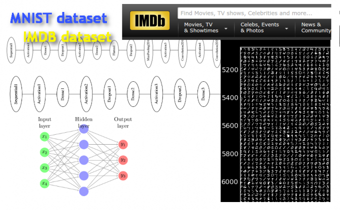
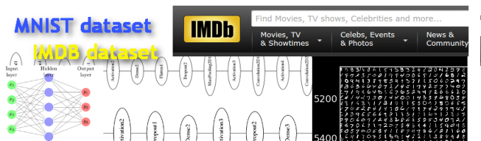
Keras and Theano Deep Learning Frameworks are first used to compute sentiment from a movie review data set and then classify digits from the MNIST dataset
Gradient Instability Problem
Neural network gradients can have instability, which poses a challenge to network design.If a network is too deep, and the weights are too small, signals will become attenuated as they move deeper into a network.The same is true of the gradient, when calculated from the output layer, and then chained into successive layers toward the input.This can make it difficult to effectively train neurons which are positioned more than several layers back toward the input. After the gradient is computed through several layers, the weights become multiplied into the gradient expression. The gradient can then become attenuated by the weights, if they are too small. This immediately leads to corrective terms becoming too small for neurons in the deeper layers, thereby making the network training ineffective by backpropagation. In others words, the training will not be able to reach far enough backward into a network. This problem is especially pronounced in recurring neural networks (RNNs), where a network’s output feeds back to its input, increasing the network’s depth.
The opposite of the attenuation scenario can also occur, where if the weights are too large, a signal will grow exponentially, and cause the network to be unstable, with corrective terms growing without bound. So how does Theano help to address these problems? If a network’s weights are too small or too large, backpropagation will not work. There is a way to balance the weights connecting the network layers, such that they do not grow too large or small. This method is called L2 Regularization, and involves adding the 2-norms of the Weight matrices to the cost function. L2 Regularization also helps to reduce overfitting to data.This, however, makes the cost function more complicated.
Successive chaining of nonlinear activation functions, such as logistic functions, hyperbolic tangents (tanh), or rectified linear units (ReLUs), along with L2 regularization leads to a pretty complicated cost function. Theano calculates the error gradient symbolically, and precisely, despite the complexity, with respect to each weight value, yielding an analytic form, which is evaluated numerically. This precision helps to eliminate numerical errors that arise in computing the gradient, using a Runge-Kutta methods. Numerical errors accumulate and worsen as the gradient is computed deeper into a network. Since each layer is connected by a non-linear function, the effect of these errors worsen. Theano produces an analytic function at every layer in a network, eliminating the accumulation of numerical errors.
The Advantage of using Theano for Developing Neural Networks
Theano makes the backpropagation training method more effective, by producing more accurate corrections for each neuron, even if they are positioned far back toward the input layer.It cannot fix a badly balanced network, but it will make the training more effective for a correctly balanced network with self-balancing mechanisms.Modern networks, such as those trained to play computer Atari games, can only remember a short distance into the past [1].
Various approaches have been considered for the initial assignment of network weights. One method is the Xavier algorithm, which balances initial weight assignments such that attenuation or unstable signal growth does not occur initially in convolutional neural networks (CNNs) [2]. The weights in this method are assigned within a uniform distribution having bounding values determined by network properties.In recurring networks, additional mechanisms must be introduced in order to prevent signal attenuation. Memory elements can be positioned in the network, where they effectively sustain signal strength at each stage of recurrence. Two memory models are the Long Short Term Memory (LSTM) [3], and the Gated Recurring Unit (GRU) [4]. The GRU is simpler in structure compared to the LSTM and has been demonstrated to perform better under certain circumstances. The LSTM model, however, has been shown to produce the best network performance given more training time, and a certain constant initial bias parameter value.
The Keras Framework
Keras puts all of these neural network features and enhancements at the developer’s fingertips. It is possible to define a training and testing set, and then train a multi-layered recurring network with LSTM (or GRU), within an abbreviated body of code consisting approximately of merely fifty to seventy lines. Keras is a high-level framework built on top of Theano.As a framework upon a framework, it provides a great amount of leverage.While Keras provides a high-level interface, it is still possible to program at the lower level Theano framework within the same body of code.
Since we will be using an NVIDIA Tesla K80 GPU card, we want to examine a network which has sufficient complexity, such that using a GPU provides some practical benefit.Simple models, or smaller components of larger networks, such as Perceptrons, Autoencoders (Restricted Boltzmann Machines), or Multi-layer Perceptrons (MLPs), do not contain enough neurons and connecting weights to require the use of GPUs.These smaller networks can instead be solved on a CPU within reasonable time. Larger networks, inspired by biological models, such as LeNet[5], AlexNet[6], GoogLeNet[7], and other deep network architectures, do require GPUs in order to decrease compute time to a practical range.Modern neural networks designed in order to do image classification, or Natural Language Processing (NLP), require a GPU [8].
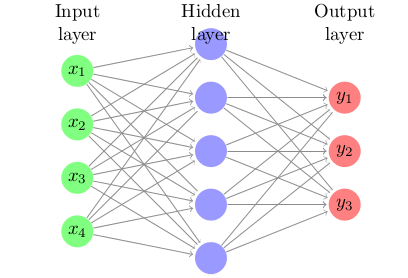
A schematic of a perceptron having one hidden layer
Using Keras, doing 1D convolutions on text data, or 2D convolutions on image data, requires about the same amount of code. The framework makes these different sorts of network convolutions relatively easy.We will examine two different types of network models: one which uses 1D convolution on textual data, and another which uses 2D convolution on image data.
We will first train a neural network on textual data contained in an IMDB movie review data set[9]. The network will then be demonstrated on a test set in order to classify reviews and categorize each as positive or negative in sentiment. In our second use case, we will create a neural network image classifier, by defining a neural network similar to LeNet5. We will train this network on the MNIST data[10], and then use the trained network to classify a set of test images.
Building a Movie Review Sentiment Classifier using Keras and Theano Deep Learning Frameworks
This tutorial will assume that you have already set up a working Python environment and that you have installed CUDA, cuDNN, Theano, Keras, along with their associated Python dependencies. The process of setting up a development environment with Keras and Theano is beyond the scope of this tutorial, but very good resources exist which explain how to do this. Using python virtual environments can greatly facilitate the task of setting up a working environment on a multi-user cluster, and is recommended. Virtual environments also make this process easier for non-administrative users who require installation of their own python packages.
To begin, you should define some Python runtime parameters in your ~/.theanorc file.
[sourcecode language=”xml”]
floatX = float32
force_device = True
device = gpu0
mode=FAST_RUN
[nvcc]
fastmath = True
[cuda]
root=/path/to/cuda
[/sourcecode]
On the node where I will build the network, there are four GPUs, numbered 0 through 3, all on NVIDIA K80 cards. Here I have selected gpu0. If you would like to compare runtimes to CPU, you can just set "device = CPU".You will also need to set floatX to be float32, along with your path to CUDA.Theano does not yet support float64 (it will soon), so float32 must, for now, be assigned to floatX.The environment variables, PATH and LD_LIBRARY, will need to be set to the correct respective directories.
On computing clusters, you will first need to log onto a node having a GPU.Logging into GPU-enabled nodes is can be done using an interactive session.
Import Keras modules:
[sourcecode language=”python”]
from __future__ import absolute_import
from __future__ import print_function
import numpy as np
np.random.seed(2222) # use the same random number seed, if you want reproducibility
[/sourcecode]
Import other needed components, such as RMSprop, Sequential, layer types, etc.:
[sourcecode language=”python”]
from keras.preprocessing import sequence
from keras.optimizers import RMSprop
from keras.models import Sequential
from keras.layers.core import Dense, Dropout, Activation, Flatten
from keras.layers.embeddings import Embedding
from keras.layers.convolutional import Convolution1D, MaxPooling1D
from keras.datasets import imdb
from keras.utils.dot_utils import Grapher
[/sourcecode]
Now some network parameters are defined:
[sourcecode language=”python”]
vocab_size = 5000#this is the number of features to use
#or, size of the vocabulary
paddedlength = 100#this is the length to which each sentence is padded
batch_size = 32#number of input batches processed per epoch
embedding_dims = 100#number of dimensions into which each vocabulary index is embedded
num_filters = 250#number of filters to apply/learn in the 1D convolutional layer
filter_length = 3#linear length of each filter (this is 1D)
hidden_dims1 = 250#number of output neurons for the first Dense layer
hidden_dims2 = 100#number of output neurons for the second Dense layer
epochs = 5#number of training epochs
[/sourcecode]
The IMDB data is loaded and stored into training, validation, and test sets:
[sourcecode language=”python”]
# split the X & Y data 80%/20% in terms of training and test data
#
(X_train, Y_train), (X_test, Y_test) = imdb.load_data(nb_words=vocab_size,test_split=0.2)
# each training and test sentence is padded to be paddedlength
#
X_train = sequence.pad_sequences(X_train, maxlen=paddedlength)
X_test = sequence.pad_sequences(X_test, maxlen=paddedlength)
[/sourcecode]
Next, the network is build by adding layers to the nn object, which is the data object for the neural network model:
[sourcecode language=”python”]
grapher = Grapher()
nn = Sequential()
# the vocab vectors for this dataset each begin as just an integer representing its frequency in the dataset as a whole
# the array of integers representing a sequence of words (or sentence) is transformed so that each word in the sequence
# is represented by fixed-size vectors, each having embedding_dims dimensions
#
nn.add(Embedding(vocab_size, embedding_dims))
nn.add(Dropout(0.5))
# we add a Convolution1D, which will learn num_filters (250) filters
# word group filters of size filter_length– here, it is 3
# the 1D convolution captures short multi-word features across the sentence
#
nn.add(Convolution1D(input_dim=embedding_dims, nb_filter=num_filters, filter_length=filter_length, border_mode="valid", activation="relu", subsample_length=1))
[/sourcecode]
A pooling layer is added to give the network some invariance to word vector position.Neural networks exhibit better performance by also training on the reverse of sentences, where the order of words are reversed, but not the letters within the words [8]Here, we train only on the original order of the sentence.
[sourcecode language=”python”]
# we use standard max pooling in 1D, halving the output of the previous layer
nn.add(MaxPooling1D(pool_length=2))
# We flatten the output of the convolutional layer
# this reduces each embedded word vector to one dimension
# this way, the output of this layer can be fully connected to a proceeding dense layer:
#
nn.add(Flatten())
# calculate the number of output neurons for this conv layer
# a "valid" type 1D convolution is sequence_length – filter_length +1
# then we divide by 2 for the maxpooling
# in the expression below paddedlength-filter_length is divided by 1 first, to refect the fact that
# the subsample_length was set to 1 as an input argument to Convolution1D()
#
output_size = num_filters * (((paddedlength – filter_length) / 1) + 1) / 2
[/sourcecode]
A fully connected layer is added with a ReLU activation function (rectified linear unit). ReLU has been demonstrated to improve the learning rate in convolutional neural networks [6]. The dropout method is used here in order to reduce overfitting to the data.When overfitting occurs, the network becomes too fit to particular details of images in the training set which do not generalize well.
[sourcecode language=”python”]
# A Dense layer is added which is fully connected to the previous convolutional layer.
# The activation function on the output of this Dense layer is set to ReLU, in order to improve learning speed.
# The hidden_dims1 here is the number of output neurons for the Dense layer.
# output_size is the number of outputs from the previous convolutional layer, or inputs into each neuron of the Dense layer
#
nn.add(Dense(output_size, hidden_dims1))
nn.add(Dropout(0.25))
nn.add(Activation(‘relu’))
nn.add(Dense(hidden_dims1, hidden_dims2))
nn.add(Dropout(0.25))
nn.add(Activation(‘relu’))
[/sourcecode]
Finally, the network converges onto a single neuron, with a logistic activation. This neuron will, after training, provide the network’s estimation of the sentiment of a text input. The network, after having been trained on a sentiment labelled set of movie reviews, is now able to evaluate sentences not previously encountered as input, and then output its computational estimate of the sentiment.It is fascinating that sentences can be analyzed in this way using one-dimensional convolution, with fairly good results, as we will see below.
[sourcecode language=”python”]
# The output layer consists of a single neuron, which is fully connected from the previous layer.
# The output signal is then tranformed with a sigmoid (logistic) function
nn.add(Dense(hidden_dims2, 1))
nn.add(Activation(‘sigmoid’))
# write the neural network model representation to a png image
grapher.plot(nn, ‘nn_imdb.png’)
[/sourcecode]
The cost function is defined here as binary cross entropy, and root mean square gradient backpropagation as the training method.
[sourcecode language=”python”]
nn.compile(loss=’binary_crossentropy’, optimizer=’adam’, class_mode="binary")
nn.fit(X_train, Y_train, batch_size=batch_size, nb_epoch=epochs, show_accuracy=True, validation_data=(X_test, Y_test))
[/sourcecode]
Finally, the network will be tested on some test samples:
[sourcecode language=”python”]
# assess the network performance on unseen test data
results = nn.evaluate(X_test, Y_test, show_accuracy=True, verbose=0)
print(‘score:’, results[0])
print(‘accuracy:’, results[1])
[/sourcecode]
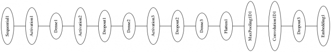
Network Diagram for a 1D Convolutional Feedforward Network Designed for the Purpose of Evaluation IMDB Movie Review Sentiment as Positive or Negative
On a CPU, the calculation requires 7864 seconds (2 hr, 11 mins, 4 seconds), resulting in 92.1% accuracy on the training set and 84.2% accuracy on the validation set, with a validation loss of 38.5%, within four training epochs.Overfitting was observed to increase beyond the fourth epoch.
Using a Tesla K80 GPU, the calculation is completed in 112 seconds, yielding essentially the same accuracies.This reflects a speedup factor of 17.6, using the Tesla K80 GPU, compared to CPU- a huge performance boost.The speedup was observed to vary according to the network architecture.Overall, it was observed to be very good for this type of 1D convolutional network.
| Neural Network Architecture | Hardware Configuration | Speedup Factor1 |
|---|---|---|
| 1-D convolutional neural network Adam optimizer | K80 GPU | 17.6 |
| 1-D convolutional neural network Adam optimizer | CPU | 1 |
1speedups are with respect to runtimes on a CPU for the respective neural network architecture.
Building an Image Classifier Using Keras and Theano Deep Learning Frameworks
Now we will turn to using Keras in order to define a neural network having an architecture similar to that of LeNet5, developed by Yann LeCun [11].This network is a convolutional feedforward network, which was, like other convolutional neural networks, inspired by biological data taken from physiological experiments done on the cat visual cortex [12].
At the input of the network, there is a square 2-dimensional input layer, 28 pixels on side.The networks consists of this input layer, which feeds into a convolutional layer, having 32 filters, each of size 3×3, with ReLU activations on outputs going to the next layer.The first convolutions layer then feeds into a second identical convolutional layer.The second convolutional layers feeds into a Max Pooling layer, which has dropout and a flattened output.The flattened output is then fed into a fully connected (dense) layer, having ReLU activation, with dropout.The final layer is fully connected to the previous dense layer with a softmax activation.
In Keras, the code for this is:
[sourcecode language=”python”]
from __future__ import absolute_import
from __future__ import print_function
import numpy as np
np.random.seed(2222)# for reproducibility
from keras.datasets import mnist
from keras.models import Sequential
from keras.layers.core import Dense, Dropout, Activation, Flatten
from keras.layers.convolutional import Convolution2D, MaxPooling2D
from keras.utils import np_utils
from keras.regularizers import l2, activity_l2
from keras.utils.dot_utils import Grapher
[/sourcecode]
Defining network parameters:
[sourcecode language=”python”]
batch_size = 128
num_classes = 10
epochs = 12
# x and y dimensions of input images
shapex, shapey = 28, 28
# number of convolutional filters to use
num_filters = 32
# side length of maxpooling square
num_pool = 2
# side length of convolution square
num_conv = 3
[/sourcecode]
The MNIST data is loaded and stored into training, validation, and test sets:
[sourcecode language=”python”]
(X_train, Y_train), (X_test, Y_test) = mnist.load_data()
X_train = X_train.reshape(X_train.shape[0], 1, shapex, shapey)
X_test = X_test.reshape(X_test.shape[0], 1, shapex, shapey)
X_train = X_train.astype("float32")
X_test = X_test.astype("float32")
X_train /= 255
X_test /= 255
print(‘X_train shape:’, X_train.shape)
print(X_train.shape[0], ‘train samples’)
print(X_test.shape[0], ‘test samples’)
# convert class vectors to binary class matrices
Y_train = np_utils.to_categorical(Y_train, num_classes)
Y_test = np_utils.to_categorical(Y_test, num_classes)
[/sourcecode]
Now instantiate the grapher and nn objects. Successive layers are added to nn:
[sourcecode language=”python”]
grapher = Grapher()
nn = Sequential()
# declare the first layers of convolution and pooling
#
nn.add(Convolution2D( num_filters, 1, num_conv, num_conv, border_mode=’full’ ))
nn.add(Activation(‘relu’))
nn.add(Convolution2D(num_filters, num_filters, num_conv, num_conv))
nn.add(Activation(‘relu’))
nn.add(MaxPooling2D( poolsize = (num_pool,num_pool) ))
nn.add(Dropout(0.5))
nn.add(Convolution2D( num_filters, num_filters, num_conv, num_conv, border_mode=’full’ ))
nn.add(Activation(‘relu’))
nn.add(Convolution2D(num_filters, num_filters, num_conv, num_conv))
nn.add(Activation(‘relu’))
nn.add(MaxPooling2D( poolsize = (num_pool,num_pool) ))
nn.add(Dropout(0.5))
nn.add(Flatten())
# three convolutional layers chained together — might work for larger images
# full, valid, maxpool then full, valid, maxpool
n_neurons = num_filters * (shapex/num_pool/num_pool) * (shapey/num_pool/num_pool)
print(n_neurons)
nn.add(Dense(n_neurons, 128))# flattens n_neuron connections per neuron in the fully connected layer
# here, the fully connected layer is defined to have 128 neurons
# therefore all n_neurons inputs from the previous layer connecting to each
# of these fully connected neurons (FC layer), reduces it’s input to a single
# output signal.Here’s the activation function is given be ReLU.
nn.add(Activation(‘relu’))
nn.add(Dropout(0.5))# dropout is then applied
# finally the 128 outputs of the previous FC layer are fully connected to num_classes of neurons, which
# is activated by a softmax function
nn.add( Dense(128, num_classes, W_regularizer=l2(0.01) ))
nn.add( Activation(‘softmax’) )
# write the neural network model representation to a png image
grapher.plot(nn, ‘nn_mnist.png’)
[/sourcecode]
The neural network object, nn, is compiled in Theano, and then trained on the validation set:
[sourcecode language=”python”]
nn.compile(loss=’categorical_crossentropy’, optimizer=’adam’)
nn.fit(X_train, Y_train, batch_size=batch_size, nb_epoch=epochs, show_accuracy=True, verbose=1, validation_data=(X_test, Y_test))
[/sourcecode]
Note here that we are using the categorical cross entropy as our cost function to be minimized.The optimizer chosen here is Adam.Adam was proposed as an optimizer method by Kingma and Ba [13]
Finally, test the neural network against an unseen test data set:
[sourcecode language=”python”]
results = nn.evaluate(X_test, Y_test, show_accuracy=True, verbose=0)
print(‘score:’, results[0])
print(‘accuracy:’, results[1])
[/sourcecode]
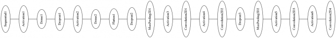
Network Diagram for a 2D Convolutional Feedforward Network Designed for the Purpose of Evaluating Images of Digits from the MNIST Data Set
Using RMSProp, the training on 60,000 samples, and validation on 10,000 samples, required 898 seconds on a CPU, using only 1 layer on convolution and subsampling.After 12 epochs, the optimization using RMSProp ended with 97.93% accuracy.There is only one convolutional layer in this network, and the number of filter features has been set to 26.
The number of filters was then increased to 32 in order to draw a comparison.The calculation takes ~18% more time to complete.With the larger number of filters, more convolutions are performed.The accuracy, however, remains essentially the same at 97.94%.The Adam optimizer was used here.Compared to the RMSprop optimization method, the Adam optimizer progresses through each epoch must faster, with a speedup factor of ~28x.
Other published results reach accuracies of over 99%.Here we are simplifying the network by removing a second convolutional and max pooling layer.When the Adam optimization algorithm is used, the accuracies are well over 97%.The table below shows various runtime comparisons using one and two-layer convolutional neural networks on the MNIST digits data.An L2-Regularization was added to the cost function.The Adam optimizer was used in computing all results in the table.
Benchmarking Results for Modified LeNet
| Neural Network Architecture | Hardware Configuration | Speedup Factor2 |
|---|---|---|
| LeNet (modified) layers: (1) 2xconv3x3 + 1xsubsampling2x2 L2 Regularization Adam optimizer | K80 GPU | 2.9 |
| LeNet (modified) layers: (1) 2xconv3x3 + 1xsubsampling2x2 L2 Regularization Adam optimizer | CPU | 1 |
| LeNet (modified) layers: (2) 2xconv3x3 + 1xsubsampling2x2 L2 Regularization Adam optimizer | K80 GPU | 33.6 |
| LeNet (modified) layers: (2) 2xconv3x3 + 1xsubsampling2x2 L2 Regularization Adam optimizer | CPU | 1 |
2speedups are with respect to runtimes on a CPU for the respective neural network architecture.
The networks in this tutorial were run on a Tesla K80 GPU. The neural networks built in this tutorial, however, can also be built using other NVIDIA GPU accelerators, such as the NVIDIA GeForce GTX Titan X, or the NVIDIA Quadro line (K6000, for example).Both of these GPUs are available in Microway’s Deep Learning WhisperStation™, a quiet, desktop-sized GPU supercomputer pre-configured for extensive Deep Learning computation.
The NVIDIA GPU hardware on Microway’s HPC cluster is available for “Test Driving”.If you are interested in testing your own deep learning software, you can request a GPU Test Drive.If you are interested in neural networks for image classification, we have more information in our blog on using NVIDIA DIGITS.
Speeding up Theano
A Python wrapper for a re-implementation of convnet, written in C++, is now available. It runs faster on GPUs, so if you are looking for a boost in speedup beyond what Theano can provide, you might want to look into pylearn2, which was also developed at the University of Montreal.
There is a method for running Theano on more than one GPU.This requires a bit of extra coding, and is described in Theano’s GitHub page on using multiple GPUs.
References
1. Playing Atari with Deep Reinforcement Learning. arXiv preprint: arxiv.org/abs/1312.5602.
2. Xavier, G, Bengio, Y. https://proceedings.mlr.press/v9/glorot10a/glorot10a.pdf.
3. Hochreiter, S, Schmidhuber, J. Long Short-Term Memory.Neural Computation 9(8):1735-1780, 1997
4. Cho, K., et al.Learning Phrase Representations using RNN Encoder Decoder for Statistical Machine Translation. arXiv preprint: arXiv:1406.1078, 2014.
5. Le Cun, Y. and Bengio, Y.Convolutional Networks for Images, Speech, and Time-Series. In M. A. Arbib, editor, The Handbook of Brain Theory and Neural Networks. MIT Press, 1995.
6. Krizhevsky, A., Sutskever, I.Hinton, G.E.ImageNet Classification with Deep Convolutional Neural Networks. Part of: Advances in Neural Information Processing Systems. 25 (NIPS 2012).
7. Szegedy, C., Liu, W., Jia, Y., et al.Going Deeper with Convolutions. arXiv preprint: https://arxiv.org/abs/1409.4842.
8. Nogueira dos Santos, C., Gatti, M.Deep Convolutional Neural Networks for Sentiment Analysis of Short Texts.Proc. of COLING 2014., Aug. 2014, pp 69-78.
9. Andrew L. Maas, Raymond E. Daly, Peter T. Pham, Dan Huang, Andrew Y. Ng, and Christopher Potts. Learning Word Vectors for Sentiment Analysis. The 49th Annual Meeting of the Association for Computational Linguistics (ACL 2011).
10. LeCun et al. (1999): The MNIST Dataset Of Handwritten Digits (Images).
11. LeCun, Y., Bottou, L., Bengio, Y., and Haffner, P. (1998). Gradient-based learning applied to document recognition. Proceedings of the IEEE, 86, 2278–2324.
12. Hubel, D.H., Wiesel, T.N. Receptive Fields of Single Neurones in the Cat’s Striate Cortex. J. Physiol. (1959) 148, 574-591.
13. Kingma, D. and Ba, J.Adam: a Method for Stochastic Optimization, arXiv preprint: arxiv.org/pdf/1412.6980v8.pdf.
14. Cowan, M. Neural Network LaTeX package, ctan.org/tex-archive/graphics/pgf/contrib/neuralnetwork.
Special Thanks
We wish to extend special thanks to Dr. Andrew Mass, of Stanford University, for allowing use of the IMDB text data set. The IMDB data set used here was originally published in [9].