In this post, we discuss how the training of deep neural networks scales on DGX-1. Considering 6 models across 4 out of 5 popular domains covered in the MLPerf v0.5 benchmarking suite, we discuss the time to state-of-the-art accuracy as set by MLPerf. We also highlight the models that scale well and should be trained on larger numbers of GPUs. Models with poor scalability should be trained on fewer GPUs, which allows for resource sharing among multiple users. As such, we provide insight into common deep learning workloads and how to best leverage the multi-gpu DGX-1 deep learning system for training the models.
MLPerf – a benchmarking suite for deep learning applications
Just as HPC system design is evolving to achieve good performance for Deep Learning applications, there is also an ever-increasing need to have a good set of benchmarks to quantify this performance. Many benchmarking tools have been proposed. For example, Baidu Research released DeepBench which focuses on basic operations involved in neural networks like convolution, GEMM, Recurrent Layers, and All Reduce. Yet there is no provision to compare different systems/workstations or even software frameworks. Tensorflow introduced TF_CNN_BENCH which is only single-domain and benchmarks only convolutional network-based deep-learning workloads. With a diversity of workloads and a variety of different hardware configurations, we need a more general approach to benchmarking deep learning applications.
With support from both industry, universities, and inspired by SPEC and TPC standards, MLPerf is a leading choice as a set of benchmarks covering different areas of Machine Learning. The goals here are multi-fold which includes a fair comparison of different hardware configurations and software frameworks, while encouraging innovation and also easy reproducibility of results.
MLPerf suite includes Image Classification, Object Detection (light and heavy), Language Translation (Recurrent and Non-Recurrent), Recommendation Systems, and Reinforcement Learning benchmarks. The suite is divided into two divisions: Closed and Open. In the Closed division the data preprocessing, training method, and model must be the same as the MLPerf reference implementation. Only very limited changes to hyperparameters are allowed. This aims for fair comparison of different deep learning hardware platforms. In the Open division any model, preprocessing, or training method can be used.
Version v0.5 received no submissions to the Open division. However, Google, NVIDIA, and Intel made submissions to the Closed division. Only Google (on cloud instance) and NVIDIA submitted GPU-accelerated results. No GPU submissions were made for the reinforcement learning benchmark, but Intel did submit a CPU-only result on Skylake processors. Software frameworks varied from Tensorflow v1.12, to MXNet for image classification, and PyTorch for the rest of the domains.
The results discussed in this post largely replicate NVIDIA’s submission in the Closed Model Division of MLPerf v0.5.0 for training. This division places restrictions on modifying hyperparameters like learning rate and batch size to provide a fair comparison of hardware/software systems. However, minor changes were required to successfully train on small numbers of GPUs. All our changes are reflected in the below log files for interested folks who want to dive deeper. We performed scaling analysis on 1, 4, and 8 GPUs on DGX-1. Our findings help deep learning practitioners and researchers determine the best options for their deep learning problem/application(s).
Training Deep Neural Networks
Training deep neural networks can be a formidable task. With millions of parameters, the model risks overfitting the training data. The deep layers in the model can have extreme gradients that lead to vanishing/exploding gradient problems. Even after accounting for all these pitfalls, the training of a network can be really slow. As a non-convex optimization problem, there can be multiple solutions and training neural networks boils down to finding a right selection of hyperparameters in order to achieve a certain threshold of accuracy. This can be done by manually tuning parameters, observing a low generalization error, and reiterating with a different combination of values until reaching the desired accuracy. When there are only a few hyperparameters, a grid search can be applied, which is more computationally intensive. A range of discrete values for each parameter is selected and the model is trained on every combination of parameters as described by the Cartesian product (grid) of the values chosen.
The following is a brief description of each model being used in the MLPerf benchmarks:
- Convolutional Neural Networks (CNN): Most widely used for image processing and pattern recognition applications like object detection/localization, human pose estimation, scene recognition; also for certain non-image workflows (e.g., processing acoustic, seismic, radio, or radar signals). In general, any data that has a grid-like topology can be processed using CNNs. Typical CNNs consist of convolutional layers, pooling layers, and fully connected layers. The convolution operation involves convolving a filter on the image, which extracts features in a local region of the image. In any image the pixels at large distances are randomly related, as opposed to smaller distances where they are correlated. The size of the filter, stride, and padding are some of the hyperparameters that need proper tuning. Pooling layers are used to reduce the number of parameters in the network, in turn reducing the number of computations. Fully connected layers help in classifying images based on the features extracted by the convolution layers. The MLPerf benchmarks Image Classification, Single Stage Detector, and Object Detection make use of a special type of CNN called ResNet. Introduced by Microsoft, ResNet [1] won the ILSVRC 2015 challenge and continues to lead. ResNets consist of residual blocks which ease the process of training extremely deep networks. A residual connection is a shortcut from one layer to another usually after skipping a few layers, basically copying the output from one layer and adding it to another layer just before applying non-linearity. MLPerf benchmarks Image Classification and Object Detection use ResNet-50 (50 layers) while the Single-Stage detector uses ResNet-34 (34 layers) as the backbone.
- Recurrent Neural Network (RNN): RNNs are interesting neural networks that offer a lot of flexibility in designing the model. It lets you operate with sequenced data at input, output, or both. For example, in image captioning with a fixed-size image input, where the RNN model generates a sequence of words describing the contents of the image. In the case of sentiment analysis, the input is a sequence of words and the output is the sentiment of the sentence: whether it is good (positive) or bad (negative). The MLPerf RNN benchmark uses the sequenced input and sequenced output model, similar to Google’s Neural Machine Translation (GNMT). GNMT has 3 components: an encoder, a decoder, and an attention network. The encoder modifies the input sequence into a list of vectors and the decoder decodes the vector into another sequence of words as an output. The encoder and decoder are connected via an attention network that allows for giving attention to different parts of the input sentence/sequence while decoding. For a more detailed description of the model, read the GNMT [2] paper.
- Transformers : A Transformer is a new type of sequence-to-sequence architecture for machine translation that uses both an encoder and a decoder, but does not use Recurrent layers like LSTMs or GRUs. Transformers are a new advancement in NLP which perform better than RNNs. A typical Transformer model would have an encoder and a decoder, with both containing modules like ‘Multi-Head Attention’ and ‘Feed Forward layers’. Since there is no RNN, there is no way of knowing the order of the words fed to the network. Therefore, we need part of the model to have a positional encoding of the words in the sequence. The source language sequence is fed to the encoder and the corresponding target language sequence is fed into the decoder, but shifted by a position. The model tries to predict the next word in the target sequence while having seen only the words prior to that position, and avoids simply copying the decoder sequence as the output. For more detailed model description, read the Attention is all you need [3] paper.
- Neural Collaborative Filtering (NCF) : Many online services (e.g., e-commerce, social networking) provide their customers with millions of options to choose from. With digital transformation resulting in huge amounts of data overload, it’s almost impossible to browse through an entire online collection. Recommender systems are needed to filter these options and help users make selections. Collaborative Filtering models the past interactions between the user and the collection. This essentially boils down to a Matrix Factorization problem where the user and collection are projected onto a latent space and the similarity (using the inner product) between the latent vectors is computed. The predictions are based on similarities. However, ‘Inner Product‘ is not a good choice of function to model complex interactions and an alternate approach of using a neural architecture to learn the arbitrary function from the data was devised. This approach is known as Neural Collaborative Filtering (NCF) [4]. Both the user and collection are represented as one-hot encoded in the input layer (sparse). A fully-connected (Embedding) layer projects this sparse representation to a dense vector. The output of the embedding layer is then fed into the Neural CF layers where each layer can learn certain structure among the interactions.
MLPerf Scaling on NVIDIA DGX-1
The MLPerf results submitted by NVIDIA make use of single-node and multi-node DGX-1 and DGX-2 systems, utilizing the entirety of the systems to train a single network. Our post discusses how performance scales when using a single DGX-1 (using 1, 4, or all 8 NVIDIA Tesla GPUs). This is important to understand how a single DGX-1 system can be used as a shared resource among multiple users, or to be used to run multiple cases of the same problem. It also helps establish which deep learning domains require the training to be done on a large scale.
Image Classification
Trained on the ILSVRC2012 dataset with 1.2 million images, this benchmark scales well. It achieves better than linear speedups going from 1 to 4 (~5x) and 1 to 8 GPUs (~10x). DGX users will achieve better throughput if they use the full system for each job.
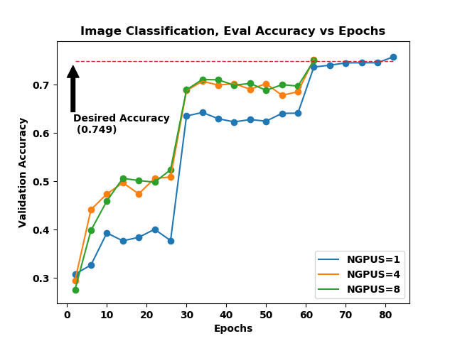
Figure 1. Evaluation accuracy vs Epochs for Image Classification.
| # GPUs | Batch Size | Average Time per Epoch (min) | Number of Epochs | Precision |
|---|---|---|---|---|
| 1 | 512 | 16.21 | 83 | fp-16 |
| 4 | 1664 | 4.56 | 63 | fp-16 |
| 8 | 1664 | 2.2002 | 63 | fp-16 |
Table 1. Synopsis of Image Classification benchmarks
Figure 1. shows the validation accuracy versus the number of epochs it took to reach that accuracy. The accuracy set by MLPerf for this benchmark is 74.9%. The 4- and 8-GPU plots achieve this accuracy in the same number of epochs, however, the average time for each epoch are different as reported in the Table 1. For a single-GPU run, the batch size needed to be reduced in order to avoid “Out of Memory (OOM)” errors. With less data being processed per epoch on a single GPU compared to 4 and 8 GPUs, it took more epochs to train the model to the same accuracy.
Object Detection – Heavy
This is the heaviest workload among all the benchmarks considered in MLPerf. Utilizing the full DGX-1, it takes ~325 minutes to train on the COCO2014 dataset. The model used is the same ResNet-50 as the Image-Classification benchmark. The speedup obtained is ~2.5x going from 1 to 4 GPUs and ~6x when going from 1 to 8 GPUs (which is sub-linear).
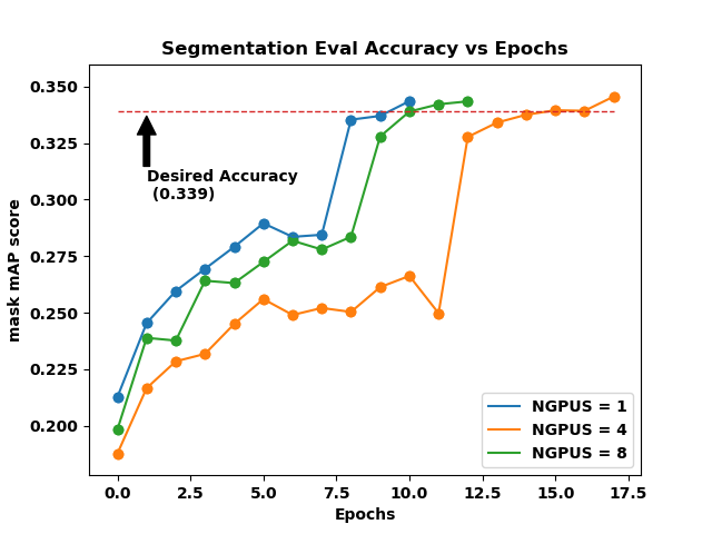
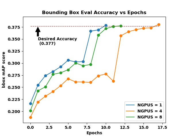
Figure 2. Mask mAP and Bounding Box mAP vs Epochs for heavy Object Detection.
| # GPUs | Batch Size | Average Time per Epoch (min) | Number of Epochs | Precision |
|---|---|---|---|---|
| 1 | 2 | 179.183 | 11 | fp-16 |
| 4 | 4 | 44.315 | 18 | fp-16 |
| 8 | 4 | 24.9895 | 13 | fp-16 |
Table 2. Synopsis of Object Detection (heavy) benchmarks
Figure 2a and 2b (click on the tabs to toggle between figures) shows the accuracy plots for the heavy object detection benchmark. There are two different accuracy thresholds here: BBOX (Fig. 2b) which stands for Bounding Box accuracy and SEGM (Fig. 2a) which stands for Instance Segmentation. Simply put, an object detection problem requires that the object be correctly located within the image and also that the object be correctly identified/categorized. Instance segmentation refers to instance of each pixel associated with an object in the image.
Object Detection – Light
The light weight object detection benchmark makes use of the COCO2017 dataset and scales with close to linear speedups: about ~3.7x going from 1 to 4 GPUs, and ~7.3x going from 1 to 8 GPUs. Total runtime varies from more than 3 hours on a single GPU to less than half an hour on 8 GPUs.
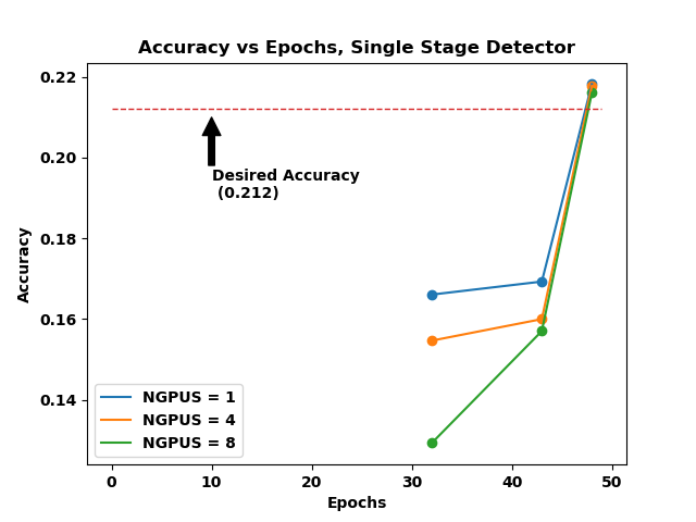
Figure 3. Accuracy vs Epoch for Single Stage Detector
| # GPUs | Batch Size | Average Time per Epoch (min) | Number of Epochs | Precision |
|---|---|---|---|---|
| 1 | 152 | 4.080 | 49 | fp-16 |
| 4 | 152 | 1.115 | 49 | fp-16 |
| 8 | 152 | 0.5628 | 49 | fp-16 |
Table 3. Synopsis of SSD benchmark.
Figure 3. shows the accuracy plots for the single stage detector benchmark. The evaluation of the model occurs only at epoch 32, 43, and 48 – hence the 3 data points in the plot. This, of course, can be modified to evaluating more often to have more data points for the plot. However, we stuck to the default values.
Language Translation – Recurrent (GNMT) and Non-Recurrent (Transformer)
The Recurrent model is trained on the WMT16 English-German dataset and the Transformer model is trained on the WMT17 EN-DE dataset. Both language translation models scale well, however transformer not only scales better but also achieves higher accuracy and averaging more in total training time.
Figure 4. BLEU score vs Epochs for Google’s NMT and Transformer Translation models.
| # GPUs | Batch Size | Average Time per Epoch (min) | Number of Epochs | Precision |
|---|---|---|---|---|
| 1 | 512 | 39.98 | 5 | fp-16 |
| 4 | 512 | 12.31 | 5 | fp-16 |
| 8 | 1024 | 6.4 | 3 | fp-16 |
Table 4. Synopsis of RNN benchmark for Language Translation (GNMT)
| # GPUs | Batch Size | Average Time per Epoch (min) | Number of Epochs | Precision |
|---|---|---|---|---|
| 1 | 5120 | 60.34 | 8 | fp-16 |
| 4 | 5120 | 22.38 | 4 | fp-16 |
| 8 | 5120 | 7.648 | 4 | fp-16 |
Table 5. Synopsis of Non-Recurrent benchmark for Language Translation (Transformer)
Figure 4a and 4b (click on the tabs to toggle between images) shows the validation accuracy plots vs epochs for the language translation models. Google’s NMT uses a Recurrent Neural Network based model and achieves an accuracy of 21.80 BLEU. The Transformer model is a new advancement in the models used in language translation which does not use Recurrent Neural network and performs better achieving a higher quality target of 25.00 BLEU.
Table 4. and 5. shows the synopsis for these benchmarks. The length of the sequence is a key parameter for a Recurrent model and does affect the scaling.
Recommendation Systems
This is the quickest benchmark to run. Even on a single GPU, it only takes a little over a minute to train to the desired accuracy of 0.635. The speedups are ~1.8x and ~2.8x when going from 1 to 4 and 1 to 8 GPUs, respectively.
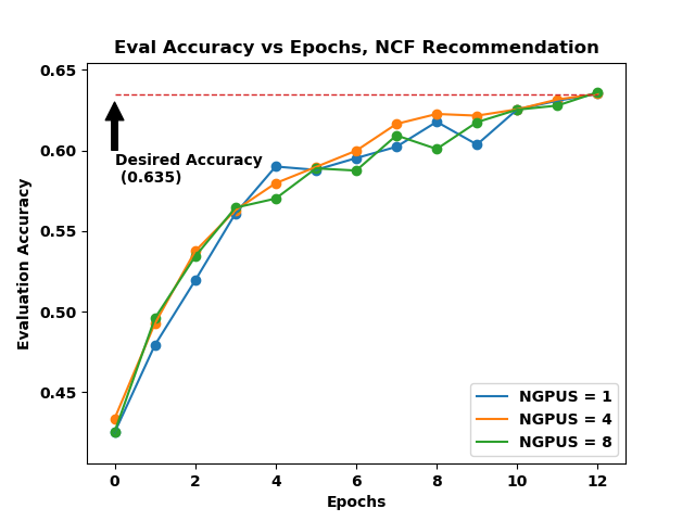 Figure 5. Evaluation accuracy vs Epochs of Neural Collaborative Filtering model for Recommendation Systems .
| # GPUs | Batch Size | Average Time per Epoch (min) | Number of Epochs | Precision |
|---|---|---|---|---|
| 1 | 1048576 | 0.135384615 | 13 | fp-16 |
| 4 | 1048576 | 0.076923077 | 13 | fp-16 |
| 8 | 1048576 | 0.048461538 | 13 | fp-16 |
Table 6. Synopsis of Recommendation Systems benchmark
Figure 5. shows the accuracy plots for the recommendation benchmark.All the plots in the figure are quite close to each other. This suggests that it’s not a cost effective strategy to use multiple GPUs for this type of workload. The benefit of using a machine like DGX-1 for such workloads is to run multiple cases, each on a single GPU. Dedicating an entire DGX-1 to a single training will reduce the training time, but is not as efficient if overall throughput is the goal.
MLPerf Scaling Results
This section summarizes the scaling results and discusses the speedups. Figure 6 (click to enlarge) shows the scaling analysis of six MLPerf benchmarks on 1, 4, and 8 GPUs on an NVIDIA DGX-1 (with Tesla V100 32GB GPUs). A general conclusion to draw from the Figure is that “all the models do not scale the same way”. Most of the models scale well. The better a model scales, the more efficiently you can train networks on large resources (an entire DGX or a cluster of DGX).
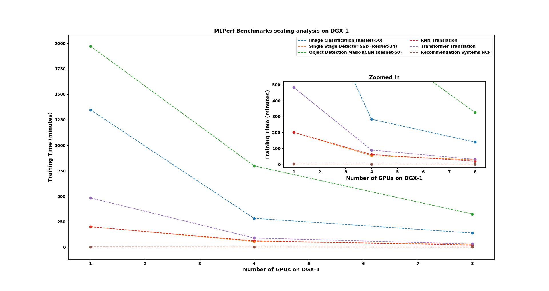
Figure 6. Scaling plots on 1-4-8 GPUs for MLPerf v0.5 Closed Model Division Benchmarks submitted by NVIDIA. The X-axis shows the number of GPUs and the Y-axis shows the training time to desired accuracy in minutes (the metric set by MLPerf). The inset axis shows a zoomed in view of the plot.
We see substantial speedups for Image Classification and Transformer Translation benchmarks (both are super-linear, running more quickly the more GPUs are added). Single-Stage Detector and Mask-RCNN Object Detection benchmark remain close to linear, while the RNN benchmark goes from linear speedup on 4 GPUs to super-linear speedup on 8 GPUs (which indicates that all of the above will scale efficiently). The Recommendation benchmark scales poorly, with fairly insignificant time savings when run on many GPUs. Table 7 lists the speedups for all benchmarks, including a calculated speed-up as the ratio of total training time on a single GPU to the total training time on multiple GPUs.
For a more detailed understanding of hyperparameters used to train these models, please reference the log files below [10].
| Benchmark | Speed Up (1-4 GPU) | Speed Up (1-8 GPU) |
|---|---|---|
| Image Classification | 4.76 | 9.70 |
| Single Stage Detector | 3.66 | 7.25 |
| Object Detection | 2.47 | 6.066 |
| RNN GNMT | 3.24 | 10.411 |
| Transformer Translation | 5.392 | 15.778 |
| Recommendation Systems (NCF) | 1.76* | 2.789* |
(*) Recommendation systems is not a good benchmark for studying scaling analysis of deep learning workloads, since it is the quickest of the bunch and the achieved speedup is on the order of seconds.
Table 7. Speed Ups for all the benchmarks going from 1 to 4 to 8 GPUs
Based on the results, a general takeaway message would be to select systems based on the type of deep learning application one is trying to build. We see that the recommendation systems benchmark doesn’t scale well, which suggests that such projects should limit multi-GPU training and instead share the resources (either shared between multiple users or between multiple models). On the other hand, if your team trains neural networks on large image sets (image classification, object localization, object detection, instance segmentation), using multi-GPU systems is crucial for quick results.
Next Steps for Successful Deep Learning Deployment
Of course, a powerful compute resource is just one part of successful deep learning implementation. Depending upon your project needs and the anticipated growth of your datasets, storage requirements may eclipse compute requirements. Connectivity also becomes critical, as neural network training stresses system and network I/O.
Whether you are planning a new project or looking to improve your existing deep learning practice, Microway’s team would be happy to help you define the requirements and deliver a successful solution. With experience in everything from GPU workstations to DGX-2 SuperPODS, our experts can ensure the deployment meets your needs. Contact an AI expert today!
References
[1]
Deep Residual Learning for Image Recognition
[2]
Google’s Neural Machine Translation System
[3]
Attention is all you need
[4]
Neural Collaborative Filtering
[5]
Deep Learning by Ian Goodfellow, Yoshua Bengio, Aaron Courville
[6]
Demystifying Hardware Infrastructure Choices for Deep Learning Using MLPerf
[7]
MLPerfv0.5 Training Results
[8]
Mask R-CNN for Object Detection
[9]
Single Shot Multibox Detector
[10]
Training results log files